Bootstrapping

Problem address

• In real life, we draw samples from our interested population, and use our samples to estimate the features of the targeted population. However, sometimes, getting samples can be expensive and time consuming. How can we know if the estimators we get from our samples are accurate for the population or not? How can we obtain more samples in a “cheap” way?

Highlights of Bootstrap:

• Resampling with replacement from your original sample data set repeatedly;
• Obtain more sample data from original data set your have;
• Quantify the uncertainty/accuracy of a statistic of interest.  Like, confidence intervals or standard deviation of your estimator.

Source book,

《An Introduction to Statistical Learning: with Applications in R》

Link to the ebook is here, https://books.google.com/books?id=qcI_AAAAQBAJ&lpg=PR2&pg=PA182#v=onepage&q&f=false

“In practice, however, the procedure for estimating … outlined above cannot be applied, because for real data we cannot generate new samples from the original population. However, the bootstrap approach allows us to use a computer to emulate the process of obtaining new sample sets, so that we can estimate … without generating additional samples. Rather than repeatedly obtaining independent data sets from the population, we instead obtain distinct data sets by repeatedly sampling observations from the original data set. ”  —- page 187 of 《An Introduction to Statistical Learning: with Applications in R》

Toy example — Estimating the Accuracy of a Statistic of Interest

Original data set dimension if 100 rows * 2 columns. 100 samples, 2 features (X and Y). Here is a scatterplot of our original data set.

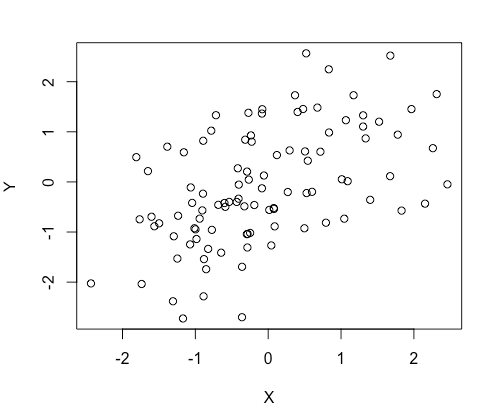
We want to use this sample to estimate the alpha value of the population we are interested in. (To stay focus on the statistic part, here I’ll skip the meaning of the alpha in the real world.)

So, our statistic of interest in this example is alpha, which can be calculated by the given formula here.    alpha = (var(Y)-cov(X,Y))/(var(X)+var(Y)-2*cov(X,Y)). We can define this function to calculate alpha in R. Later I will paste the script below.

Using the original data set, we can only calculate 1 alpha value, let’s name it alpha0.

Here comes the question we addressed at the beginning of this article.

How can we know if the estimators we get from our samples are accurate for the population or not? How can we obtain more samples in a “cheap” way?

First, let generate 1 brand new sample data set from our original data set with the same number of samples. Let’s say you have 100 samples.

The approach is simple, sample from your original sample data set with replacement. Then you will have a brand new data set with 100 samples. With this new data set, you can calculate 1 alpha value, let’s name it alpha1.

You can repeat the above step with number of arbitrary times, to generate a bunch of new sample data sets. As a result, you will have a bunch of alpha values calculated from them. Let’s say, you set the arbitrary times as 1000 times.

Then you will have 1000 new alpha values. I can plot the histogram plot of this 1000 new alpha value below. The read line marked the alpha0 value calculated from your original data set.

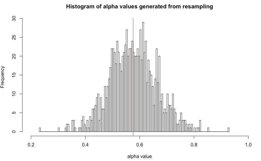
From the 1000 new alpha values, you can do a lot of things to estimate how accurate your alpha0 is.

Here are a few analysis you can do, calculate the standard deviation of your alpha, calculate the confidence interval of your alpha.

Now you can answer the 2 question above now. You can use the confidence interval calculated to say weather your alpha0 lies inside. And using standard variation to describe how variated your estimated alpha can be. The approach is named bootstrapping.

Toy example’s R script

Most commonly used function regarding to bootstrapping in R is, boot();

library(ISLR)
library(boot)
data(Portfolio)
alpha<-function(original_data, index){
 X<-original_data$X[index]
 Y<-original_data$Y[index]
 alpha<-(var(Y)-cov(X,Y))/(var(X)+var(Y)-2*cov(X,Y))
 return(alpha)}
boot_result<-boot(Portfolio,alpha,R=1000)
plot(hist(boot_result$t, freq = F, breaks = 100), main=c("Histogram of alpha values generated from resampling"), 
 xlab=c("alpha value"), xlim=c(0.2,1))
abline(v=alpha(Portfolio),col=c("red"))